I- 6-1 Zeta function
I- 6- 2 Gamma function
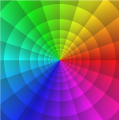
I-6- 3 W.F. Sierpinski curves -complex numbers
I- 6- 1- Zeta function
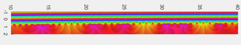
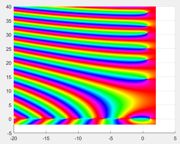
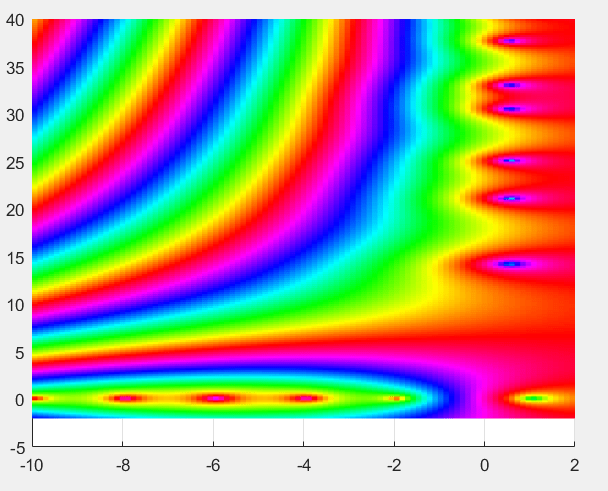
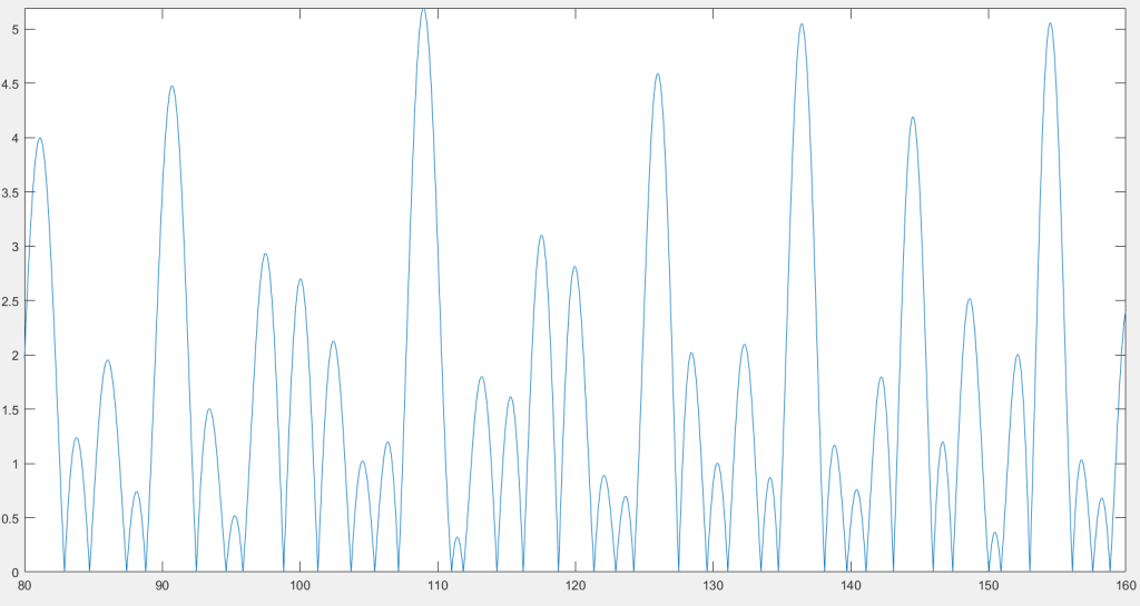
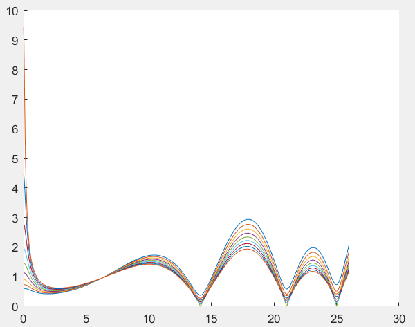
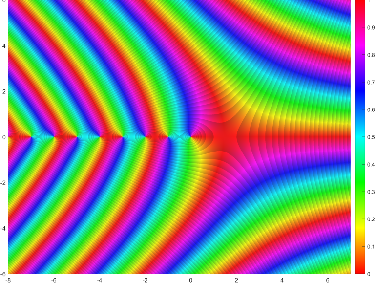
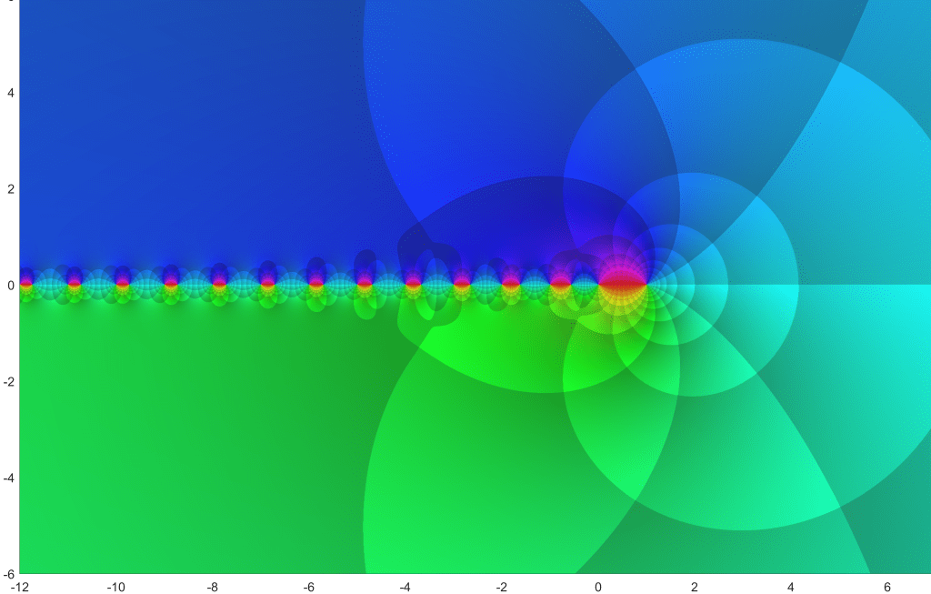
https://complex-pictures.com/i-5-potenzieren-mit-wurzel-1-i/When you use and think about complex numbers, you come to Bernhard Riemann (1826-1866) and his basic works on the zeta-function. We begin with a phase portrait of it (s.Lit.(1) p. 202, 214) , see Wipikedia ‚Riemann‘ Zetafunktion‘ and we work on the following question: is it of any use to operate with –to the power of -i- to get a clearer presentation of the trivial and non trivial zeros? It is our opinion that the ‚blue‘ spots in fig.1,3,5,7 represent such zeros.
Even if you add up the definition zeta-sum to 4000, you receive only a poor picture of the function. Zeros at 14.2 , 21.1, 24.9, 30.3, 33.1 and 37.7 could roughly be seen but they are numerically not precise and show additional false ‚zeros'(Lit(1),p202,214). To calculate the following portraits we used matlab (R), other computer languages like Wolfram Alfa (R) do these calculations too. 40.000 calls of the zeta commands affords a relatively long calculation time (> 4 – 5 Min).
Wer sich mit komplexen Zahlen beschäftigt, kommt an Bernhard Riemann (1826-1866) und seinen Arbeiten zu der Zeta-Funktion nicht vorbei. Beginnen wir mit einem Phasen-Portrait der Zeta-Funktion (vgl. Lit(1) S.202 u.,214 ; und Wipikedia ‚Riemann Zetafunktion“ ) und der Frage, ob das Potenzieren mit i eine übersichtliche Darstellung der trivialen und nichttrivialen Nullstellen erlaubt. Unserer Meinung nach stellen die ‚blauen‘ Punkte in Abb.: 1,3,5,7 Nullstellen dar.
Selbst bei der Summe bis 4000 in Abb.: 1 ergibt sich nur eine sehr unvollkommene Annäherung an die Funktion (Lit(1) S.215) . Nullstellen um 14,2 , 21,1, 24,9, 30,3 , 33,1 und 37,7 mit x ca. 0.65 deuten sich zwar deutlich an, sie sind allerdings numerisch ungenau und es gibt zahlreiche Falschsignale. Die Funktionsberechnungen der folgenden Phasenpotraits wurden mit Matlab (R) vorgenommen; auch andere Programmsysteme z.B. Wolfram Alpha, berechnen die zeta-Funktion für den Zahlenbereich komplexer Zahlen. Für 40.000 Berechnungen der Funktion wird die Computer-Belastung jedoch erheblich ( >4-5 Min).


I- 6- 2 Gamma function, ( Γ )
Lit(2) Handbuch der Theorie der Gammafunktion , 1906 , Dr. Niels Nielson, Kopenhagen .

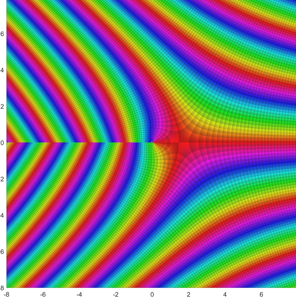

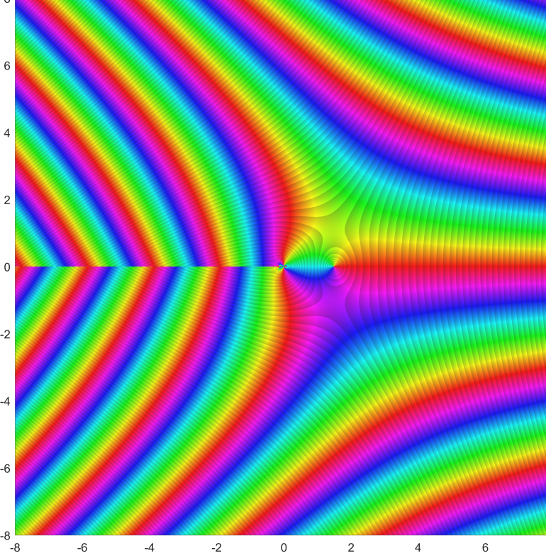
Fig. 13: f = sqrt(2pi) *(exp(z)*(z^(z-3/2)*(z-1/2) + z^(z-1/2)*log(z))*(1/(12z) – 1/(288*z^2) +1) – z^(z-1/2) *exp(-z) * (1/(12*z) – 1/(288*z^2)+1 -z^(z(-1/2) * exp-z)*(1/(12*z^2) – 1/(144*z^3)) ). – derivative formula produced by matlab (R) symbolic toolbox-. (Here it is the derivative built ‚by hand‘ without correction terms:
Γ ‚ =sqrt(2pi) *(exp((z-1/2)*log(z))*(log(z)+(z-1/2)/z )*exp(-z)) – (exp(-z))*(exp((z-1/2)*log(z)))
The phase portrait of the Euler/Mascheroni/Weierstrass definition f = exp(-0.577216*z) / z * Π exp(z/n) * (1+ z/n )^-1 is as assumed totally identical, but the computation times are much longer.
In Wikipedia some phase portraits of the zeta- and gamma function as well as of their derivatives were presented, they came from Wiki – Common. Unfortunately no detailed information of the used formulas for these pictures were given. The authors called themselves ‚ Rumil ‚ or ‚ Empetrisor ‚ .

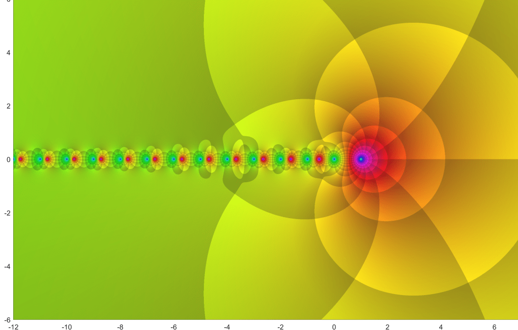
Fig. I- 6- 16 / 16a Γ`/ Γ Phi-function or Digamma – function to the power of i , f = – Σ ( 1 / (z + n) – 1/ (1 + n)), n=0:2000, left rotated.
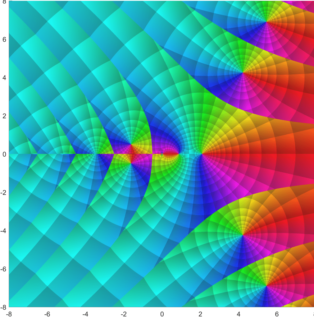


We cannot detect any severe differences between gamma and 1 over gamma in this projection.

1. Derivative of gamma function ; Γ(z)/ Γ(z) = (here called Phi - function multiplied by gamma function , results in Γ(z; see Fig . 15 and 14 , 2.200*2.200 pixel . This picture is also shown in Wekipedia ‚Gamma-Functioen‘ (author ‚Empetrisor‘). It reveals that the derivative of the Stirling approximation in Fig.13 yields only a poor picture of the function fig. 20 .

In summary both groups of functions of section I- 6- mostly do not really contribute to attractive pictures to this website. The zeros of the zeta -function are clearly visible but not always to the wanted extent of focus. We feel that only Fig. 16 and 17 are prominent examples to see the zeros more clearly.

Γ “‘ = (Γ ‚/Γ)‘ ‚ * Γ
+ 2*(Γ'/Γ)'*Γ` + (Γ ` / Γ) * Γ “ . With the obtainable derivatives of the poly gamma functions it is straight forward to calculate all derivatives of the gamma function.I- 6- 3 Waclaw Franciszek Sierpinski ( 1882 -1969)
Lit: .R.L.Devanay Cantor and Sierpinski . Julia and Fatou. Complex Topologie meets .Dynamics. Notes of the AMS 2004, p 9-15 .

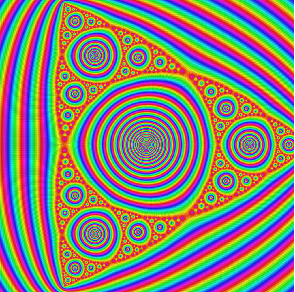
Fig. 24 . Here we see the famous Serpienski triangle. F(z) = z^2 – 0.593 / z . (see also http://www.mathe-kalender.de 2018 , September , E. Weigert et al. and cited literature therein) . Fig.25 (right) shows the function to the power of – i – .
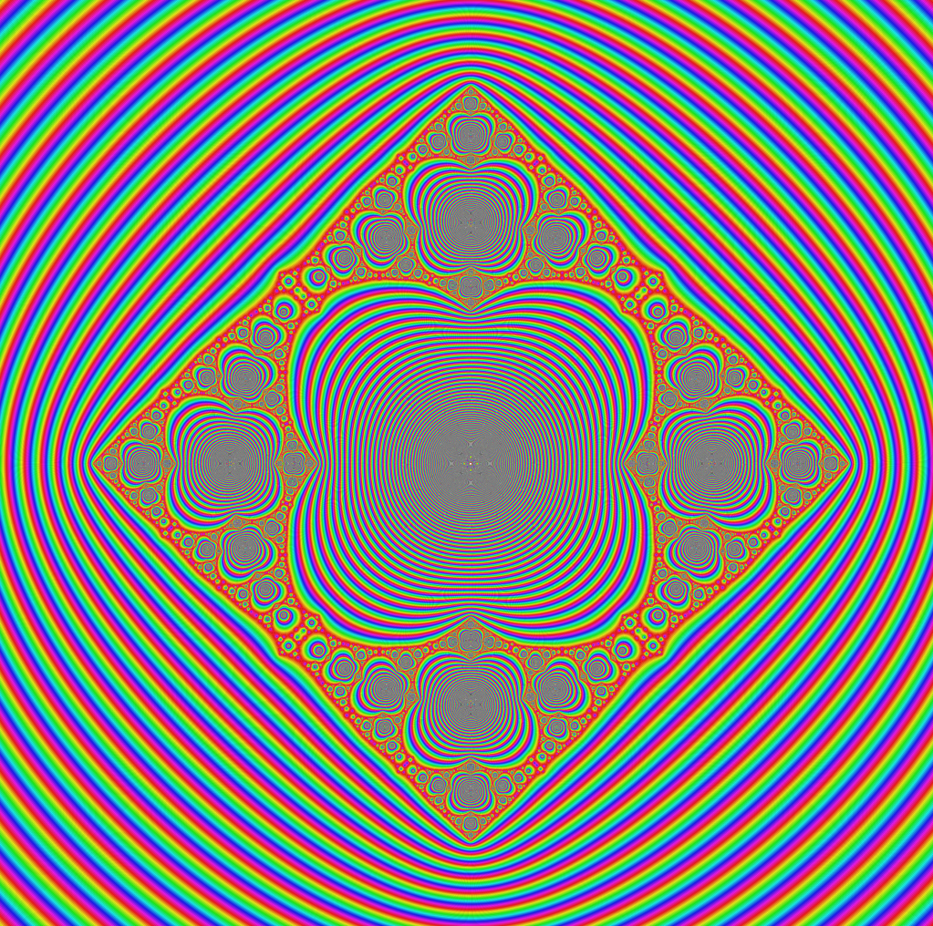


Fig. 26 -28 : Do we have here tree further Sierpinski figures ? All fig 26- 29 have a 6 fold iteration
Fig. 26 f(z) = ( z^2 – 0.34 / z^2 ) ^i .
Fig. 27 f(z) = ( z^2 – 0.2 / z^3 ) ^i .
Fig. 28 f(z) = ( z^-4 – 0.65 / z^-2) ^i .
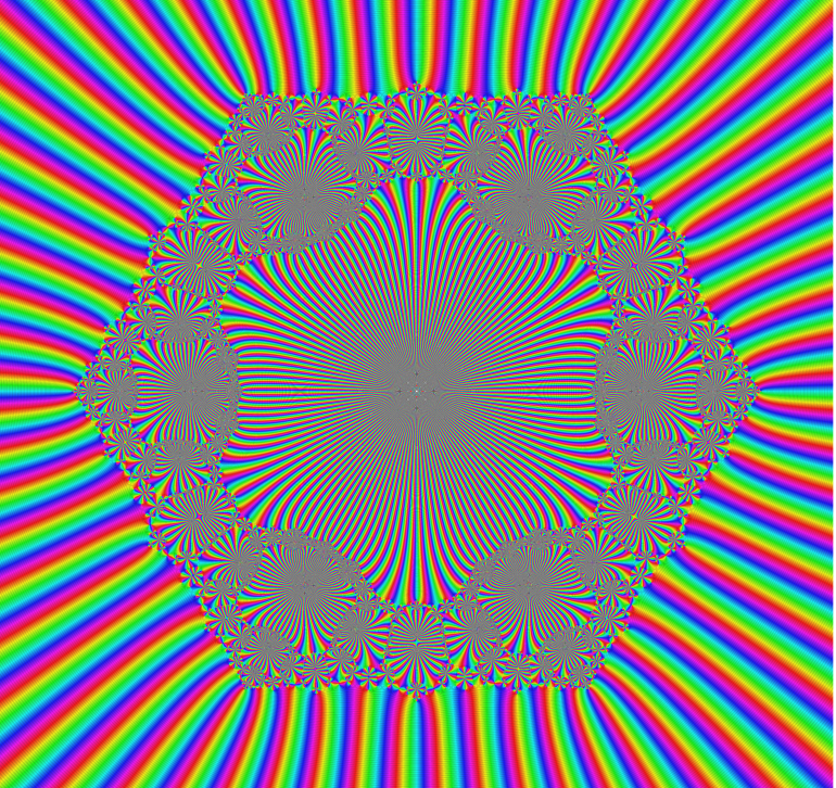
Fig. 29 f(z) coresponds to Fig 28 without ^i .
